

Excel Conditional Formatting Practice Questions
In the previous blog, we practiced some basic questions on MS Excel formatting and filtering. In this blog, we will look at Excel conditional formatting practice questions.
if you want to practice more Excel questions, visit Excel Basics to Advanced Practice Questions.
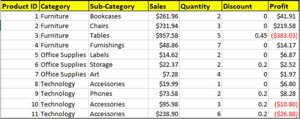
Ques 1. Using the data set given in the previous blog, change the formatting of the values in the Profit column. Negative values should be displayed in red color and in parenthesis.
Output:
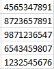
Ques 2. Using the list of numbers below, format them as phone numbers.
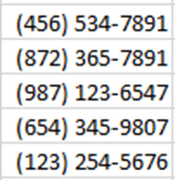
Output: After tformatting the above numbers, your output should appear like the one shown below.
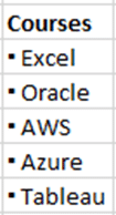
Ques 3. Use the list courses shown below, format them so that a bullet icon appear before them.
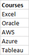
Output: After you have completed your changes, the output should appear like the one shown below
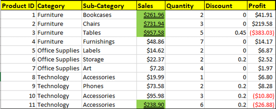
Ques 4. Use the output of Ques 1 as the dataset for this question. Format the Sales values in such a way that Sales greater than 200 is highligted in green color and is double underline.
Output:
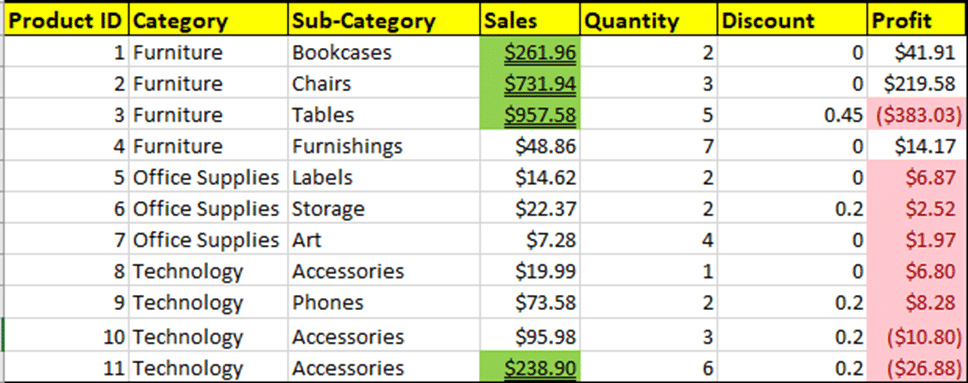
Ques 4. Use the same dataset as shown above. Highlighed Profit less than $10 in red color.
Output:
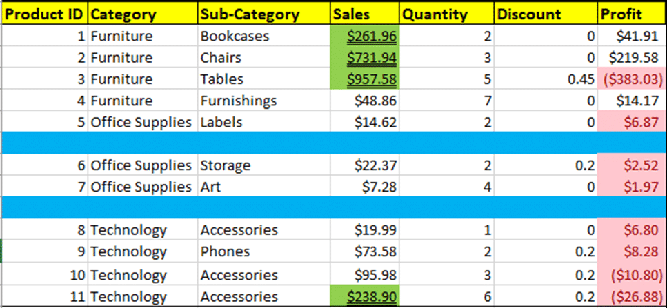
Ques 5. Insert two blank rows in the above data set. Create a conditonal formatting rule to highlight the blank rows in blue.
Output:
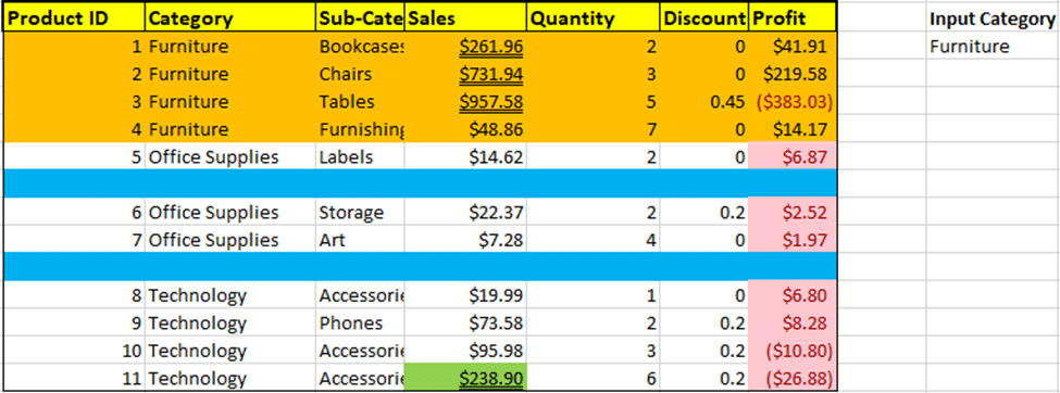
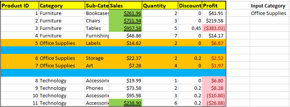
Ques 6. Use the above dataset. Create a column on the far right to Input the Category values. Start with Category = Furniture. When Furniture is entered, all the rows in the dataset pertaining to Furniture should highlight in brown. When anyother value is entered for the Category, those rows should get hightlighted.
Output: When Category Furniture is entered for Input Category
Output: When Category Office Supplies is entered for Input Category
For a step-by-step approach to learning more advanced features and functions in Excel, take a look at the book Excel Basics to Advanced.